Rob Welch

Before starting my PhD in October 2016, I helped the FFEA team at Leeds polish up their software and release it to the public. Over the next two years, I continually improved the software in parallel with my research. This post is about my improvements to the software!

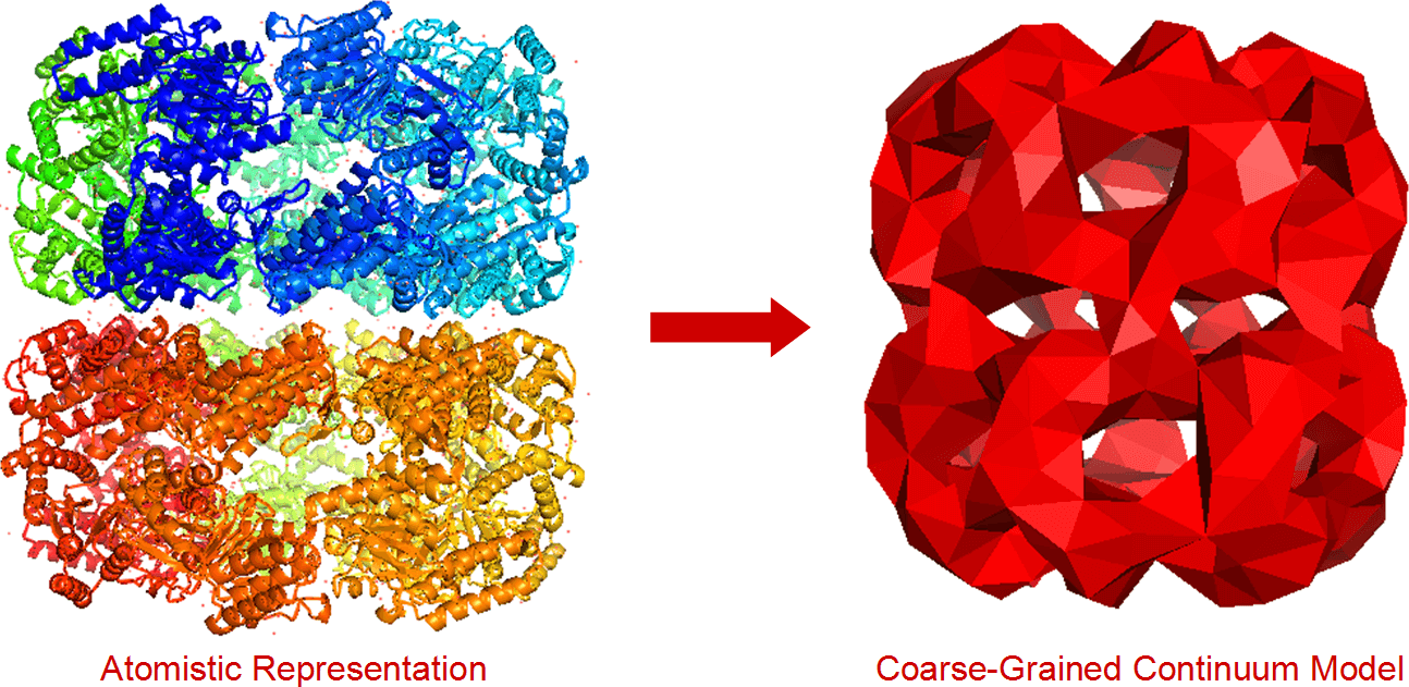
FFEA (more info here) is a continuum mechanics biophysics simulation package designed to simulate large, complex systems of biomolecules. It had been in use at Leeds for a few years (mostly for simulations of the motor protein Dynein), but the team wanted to release it as free software.

Documentation

I wrote the first version of the FFEA installation guide, along a quick tutorial for our python API, and another for visualisation using our PyMOL plugin. I can’t take the credit for the software being easy to install, though, that goes to Albert Solernou.

Additionally, I created a basic website for the project, and started hosting our documentation online – previously, users would have had to compile the software in order to have this documentation, which creates this horrible chicken-and-egg installation situation. For fun, I reskinned Doxygen to make it a bit easier to read, and in keeping with the look of the rest of the FFEA website. Later, Albert was able to set readthedocs to automatically host documentation when new versions of the software were released.

Structural improvements

FFEA is a multi-language project, comprising two big slices of C++ and Python, and a small slither of C. Most of the C++ code just fed into one big statically-linked executable with some fairly simple command-line arguments. From a user’s perspective, nothing could be easier. However, the FFEA tools, a suite of initialisation and analysis tools written in a mixture of Python, C++ and C, were in worse shape. They mostly existed as a collection of disparate scripts, scattered around the install directory. It was possible to run them using a ‘launcher’ script, which ended up being on the system PATH, but this was a bit hack-y (I think we had 2 simultaneous command-line wrappers going at once).

I decided that I would unify these scripts, along with some of the self-contained C++ executables, into a more consistent API. This would mean less duplication of code between scripts (there was a lot!), it would make the FFEA tools easier to extend and enhance, and it would make it easier for users to install and use them – ideally, they should be usable in a python interpreter just by typing ‘import ffeatools’.

I also strove to make the existing command-line interfaces more consistent. I stripped out the custom sys.argv sniffing code (again, duplicated but slightly different in each file) and replaced it with a more standard use of the python argparse module. However, these scripts also needed to be imported as a python package, so they gained the ability to detect whether they were being used on a terminal or in a package, and adapt themselves to either. Furthermore, the most important C++ and C scripts gained python wrappers, so that they could all be used from one, unified interface.

These improvements also permitted the creation of the ‘FFEA meta’ object. An instance of the FFEA meta class is automatically created when the FFEA tools are loaded, and can record the parameters being given to all of the different FFEA scripts using a few simple hooks. It will also automatically write that information to a file, and name that file in line with the other FFEA files. The end result is that the user doesn’t have to worry about manually writing down or losing their initialisation parameters. This object would not have been possible without packaging!

I also rewrote the FFEA error handling code in its entirety. Previously, all of the code had suppressed error messages. I think it’s better for the user to see what the error is, so I edited huge swathes of error handling code to re-raise the original error along with a helpful message. I also removed a number of instances of ‘error handling as control flow’ and replaced them with verbose errors with the correct exception type. That said, there are a few cases of ‘non-pythonic’ error code left, notably in the file IO scripts, as asking for forgiveness (as in ‘whoops, I tried to read a line out of a file that didn’t exist, guess I’m done’) is a lot faster than asking for permission.

Finally, I fixed a number of bugs, most of which were related to the visualisation tools, file IO (particularly parsing PDB files), deprecated code, and the installation process.

Viewer enhancements

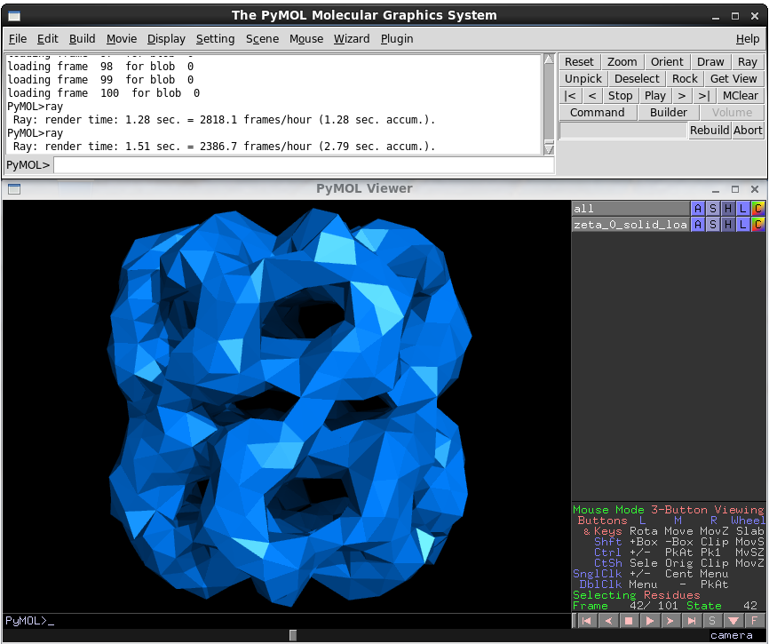
Since the end of my work on my undergraduate project, the homegrown FFEA trajectory\molecule viewer had been deprecated in favour of a plugin for PyMOL, the python molecular dynamics viewer. This viewer was brand new, and was pretty bare-bones.

First, the viewer was unstable. When it didn’t core dump due to a thread safety issue, it would throw up exceptions due changes in the FFEA python modules. The former issue was actually quite easy to fix – the viewer relied on loading the FFEA trajectory information on a separate thread to the renderer for the main window (in order to keep the viewer responsive). The fix was to use a drop-in replacement for the Tkinter library, called mtTkinter, which automatically handled threading, and stopped the majority of crashes (I have no idea why this isn’t shipped with Python instead of Tkinter). As for the latter, hitting this moving target eventually drove me to write unit tests for the core FFEA modules, something that is still ongoing.

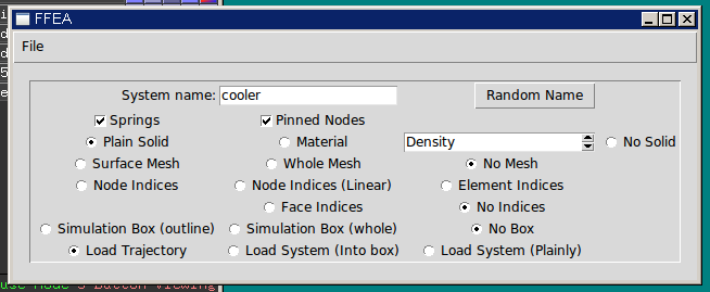
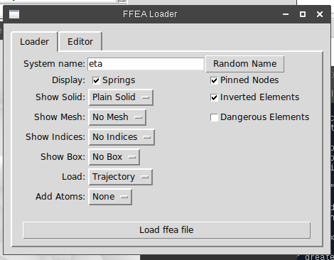
After that, I decided to tidy up the user interface for the PyMOL plugin. At the time, this consisted of a collection of radio buttons with not-very-descriptive labels, thrown into a window seemingly at random (they weren’t even lined up!). This is fine if the software is only for internal use, but now that it was going public, I made an effort to group the controls in a structured and logical fashion, and label each group.

I also added a few features. The first was the ‘CGO’ trajectory loader option. PyMOL accepts input in the CGO format, which lets you feed vertex data into it as a series of huge strings of numbers. These strings are formatted as a series of control codes (indicating whether the data forms a triangle, line, cylinder etc) followed by the positions of the vertices, and the vertex normal vector (needed for lighting).

Here is where the problem lies: the FFEA data files are not structured in this way. The nodes are saved in one file, and are loaded into quite a complex, hierarchical object. In the file, and the object, there is no way of knowing which vertex each node belongs to. That information is given in the surface file\object (or the topology, as interior nodes form tetrahedrons, not triangles). Each vertex contains 3 nodes, but each node belongs to 3 different vertices, meaning that each node has be loaded three times. This has to happen for each frame in the trajectory. So, 100 frames of 1000 nodes doesn’t sound like much, but it means that 300,000 lookups have to be performed, along with a few tens of thousands of vertex normal calculations, which can take quite some time.

I wish I could say I’d written some incredibly clever algorithm that does all of this much faster, but the reality is that no amount of clever algorithms can ever match up to that time-honoured tradition of cheating.

I rewrote the trajectory loader for special cases like this. Rather than loading into a complex object, it wrote all the data into a monolithic n-dimensional array. This meant that reading in the data was only bottlenecked by the speed at which the program could iterate over the lines in the file. Next, the array was cached to the hard drive in a binary blob (normally making it orders of magnitude smaller than the trajectory file itself, which is a text file). Then, the surface normals and calls to CGO were pre-calculated and also cached to the hard drive. Because they’re now accessing this monolothic array object, everything is a little faster. And because they’re cached, loading the file is instantaneous (after the initial generation).

This method isn’t much faster for a regular trajectory, but for extremely large trajectories, it’s extremely fast. This was an utterly useless feature for about 2 years, but as of 2018, Tom Ridley has been using FFEA for colloid simulations that involve thousands of objects, and the standard FFEA trajectory loader runs out of memory long before loading in an entire trajectory of these objects. On the other hand, loading them with the new CGO loader is fairly fast.

Now that the way was paved to make the viewer more ‘interactive’, I looked at trying to add useful features (both for potential users of the software post-release, but also for the rest of my PhD!). First on the list was tracking element inversions. The simulation will often crash when a certain element ‘inverts’. This happens when a tetrahedron undergoes enough force to literally turn it inside-out. The result is that the element has a negative volume, and this cause the numerical integration function (which uses the Euler method) to become unstable. Luckily, when this happens, the software will tell you which element inverted. The problem is that there was no way of visualizing that element in the PyMOL plugin. Element indices could only be displayed as 3D models, and even then, you’re going literal needle-in-a-haystack mode.

I designed two features to completely address this. First, the user can specify a number of nodes in the user interface to be highlighted. The software will then generate specific CGO ‘objects for those nodes, and put them in a separate PyMOL object. Then, the user can set the colour of that pymol object to whatever they like.

Second, the user can push another button (‘Add node indices’) at any time to have ‘psuedo-atoms’ generated at the location of each node. While you can draw objects into PyMOL quite easily, none of PyMOL’s measurement techniques actually work on them (e.g. if you want to measure the distance between two nodes). Generating psuedo-atoms fixes this – and if you set the name attribute to the index of the atom, then you can view their names or target them using a few commands in the pymol console.

I feel the need to point out that if you’ve used any of these tools whilst using the FFEA viewer, you should definitely also thank Albert Solernou, who took a lot of time to upgrade and improve them before the official launch of the software. He and Ben Hanson also added tools to alter surface-surface interactions in realtime.

FFEA automodel: training wheels for tetrahedral mesh generation

Mesh generation in FFEA has always been something of an inconvenience. It’s the first thing that the user does, but it’s mediated by about 6 different command-line tools made by different people in different languages which often don’t work. These tools are powerful and capable in the hands of an experienced user, but for a new user they can be somewhat overwhelming. You know why WordPress is popular? It’s because you can install it in 5 minutes. Jenkins? Same deal. Albert had been working on the 5-minute install, where dependencies were automatically downloaded and statically linked against the FFEA executable, so I wanted to do the same thing for model generation.

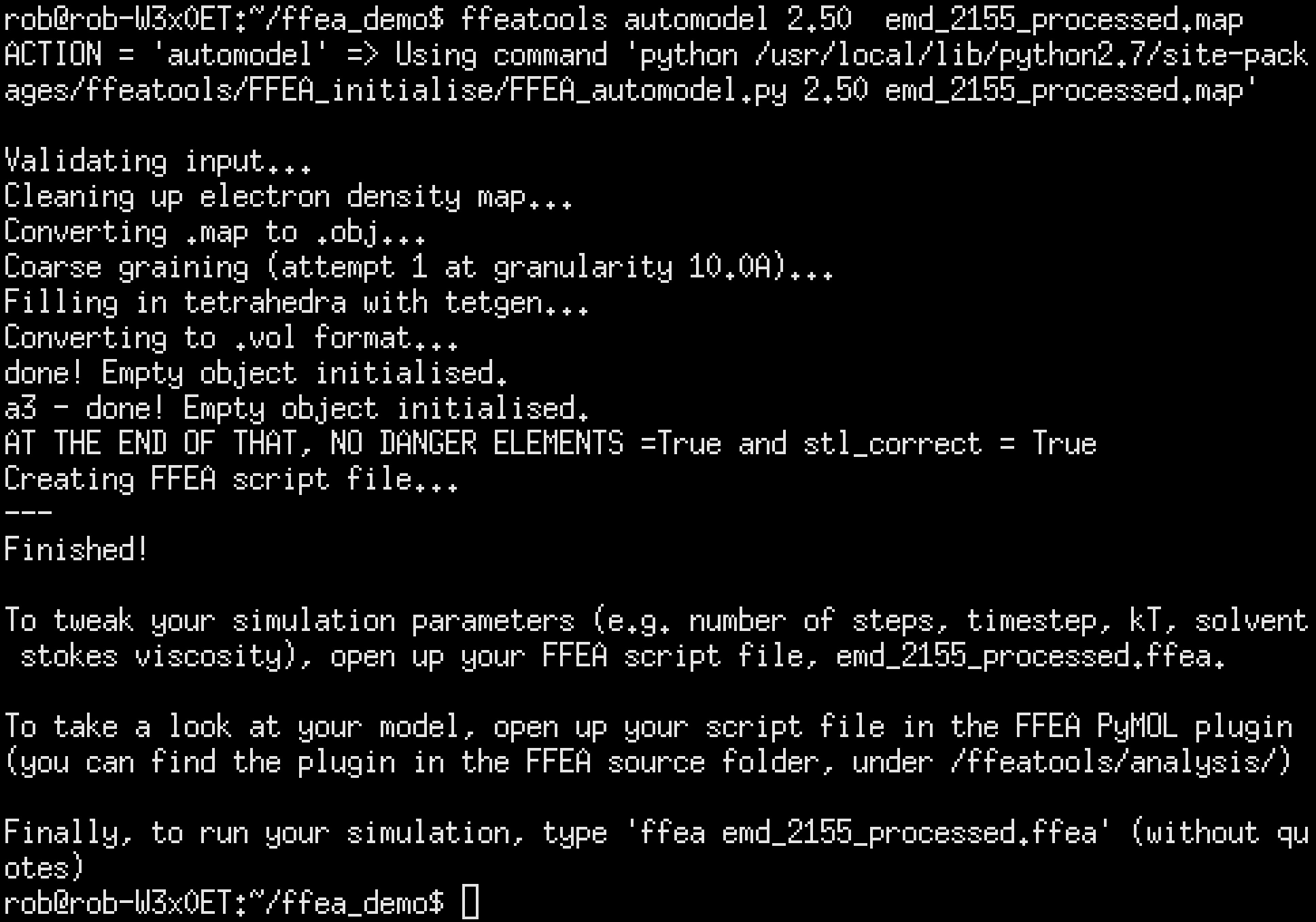
The tool I came up with was FFEA automodel. Here’s the feature list:

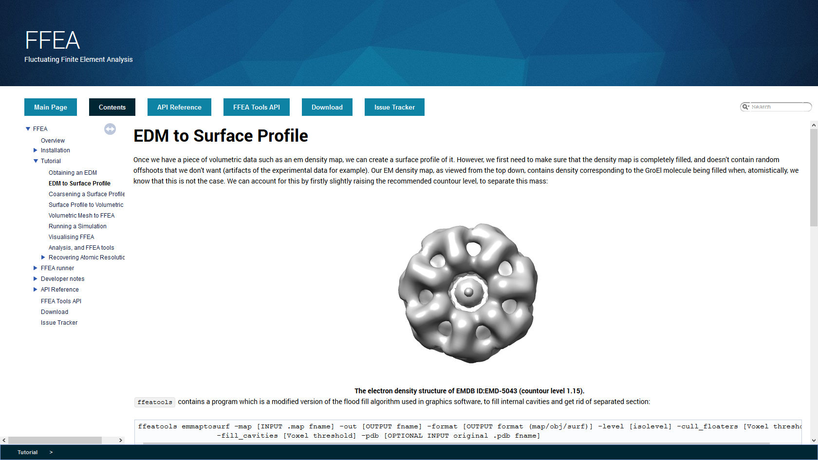
• It ferries data to and from different command-line utilities without the user having to get involved. It starts with an EM density map, which it converts to a surface mesh, coarse-grains the mesh, fills the mesh in with tetrahedra and converts it to an FFEA-compatible format with an FFEA script file.
• It inspects the input given by the user to make sure it’s sensible and won’t break anything. It checks the granularity and the material parameters (the two things which can cause a simulation to become numerically unstable) and also checks that the various FFEA packages have been correctly installed, and that the input is a valid format. It even checks that the user has the correct version of Python installed.
• It inspects the output given by these utilities to make sure that they’ve help up their end of the bargain as well. It checks both the obj file spit out by the electron map to surface converter in order to ensure that the ISO level has been set correctly, and it checks the area and length of the tetrahedra generated to ensure that none of them are too small or too thin. If it does detect this, it will attempt to coarsen the further, in 1A increments, and if problems still persist it will politely inform the user as such.
• It provides sensible default values for (almost) all the quantities involved. Granularity, material parameters, smallest element thresholds, small object culling, etc. The only thing it doesn’t provide a default for is ISO level, because that’s entirely arbitrary and always given by the EMDB map author.
• It points the user where to go next, and gives them advice on how to fix their input files if things go wrong.

Automodel is distributed with new builds of FFEA, and I’d highly encourage you to give it a try, particularly if you’re not proficient with Linux or with preparing meshes for finite element models.

Seemingly unending self-promotion

I go to people and talk at them about FFEA. Hopefully in nice places, not Manchester. Here’s my standard diatribe!

Validation for the FFEA software publication

I didn’t write any of the FFEA software publication, my name was really on there for the work I’d done on the software, some of which I’ve detailed here. Of course, my main job is Cosserat rods, but I’ll save that for another post. When the paper came back from review, some of the reviewers noted that they’d like to see a comparison between FFEA and atomistic molecular dynamics.

This is problematic for many reasons, the main one being: FFEA is designed for large, mesoscale systems, operating on very long timescales. It would not be easy for us to run our own atomistic MD simulations, especially given the short timescale we had. I was drafted in to fix the problem by Albert Solernou, who suggested I look at the MoDEL database. This database contains reference trajectories for many biomolecules, normally very long and compressed using Principal Component Analysis (PCA). Think of it like this: when a biomolecule is fluctuating in thermal noise, what it’s really doing is a series of fluctuations with a very consistent period about a bunch of different axes. Some of these so-called ‘bending modes’ are large, representing the entire molecule moving back and forth, and some are small. It might bend more in one axis than another. Principal Component Analysis takes a regular trajectory and decomposes it into these modes, and is a highly efficient way to store this information without that much loss of data.

Albert suggested a range of molecules to use that would represent different kinds of motion. I ended up with one molecule which was long and thin, with the kind of large-scale motion which FFEA would be good at representing, and another whose motion depended mostly on internal atomic fluctuations, so which would not be so well-represented by FFEA’s ultra-coarse approach.

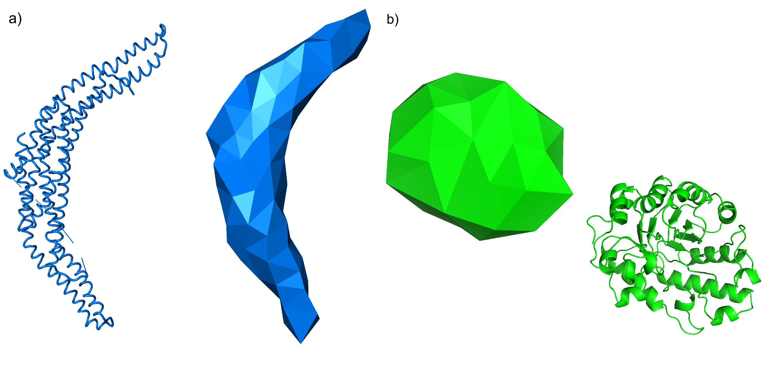
The boomerang-shaped thing on the left is Arfaptin and I have no idea what it’s for. The blob-shaped thing on the right is Xylanase, and I have no idea what it’s for. However, I did have the principal components of both. I generated FFEA meshes and ran FFEA simulations of both molecules for a period of at least 10 microseconds for each molecule. In a PCA comparison, we use the dot products of the eigenvectors that represent the principal components of the motion, and there’s one eigenvector for each node in our system. This is bad news for us, because the two systems have a different number of nodes (each FFEA tetrahedron represents a number of atoms, maybe like 10 or 20 in this case).

Now, Ben Hanson had written a program to map FFEA trajectories back onto atomistic structures, interpolating the positions of arbitrary points inside the tetrahedra. The issue was, the PCA trajectories were aligned differently to my own. The starting positions of the two sets of atoms must be the same, otherwise the dot products will be wrong.

Arfaptin was easy enough, it could be aligned by visual inspection. Xylanase, however, could not – especially as the only alignment tools we had at the time were tedious, command-line tools which required the user to reload the visualiser when they made a change. To align the the Xylanase trajectories, I created a new tool, node_pdb_align, which would align entire trajectories using the iterative closest point algorithm. This tool was based on an implementation of the algorithm by Clay Flannigan in Python. It’s effectively a minimisation algorithm, but instead of energy you’re minimising the RMSD. It does tend to get stuck in local minima, so I modified it to start from a set of random starting positions. It’s now part of the ffeatools package that comes with FFEA.

With PDBs aligned, I was finally able to compare the trajectories, here are the results:

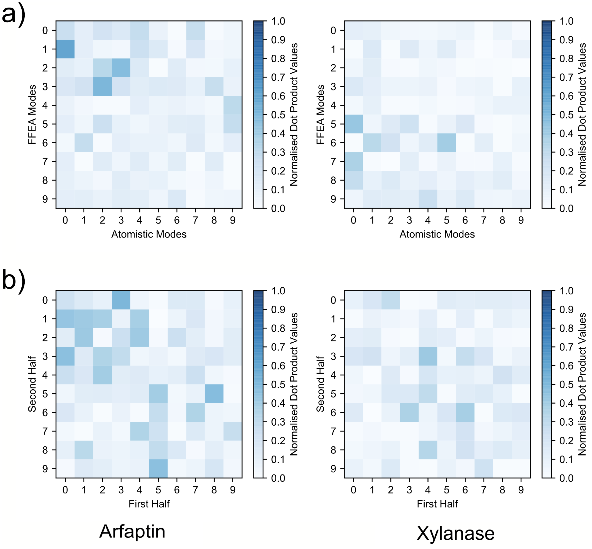
The top two figures show the dot product matrices of the atomistic trajectories with the FFEA trajectories. If the two trajectories were entirely identical, you’d see a perfectly diagonal blue line. What you see is a vaguely diagonal blue cloud. That’s where the bottom half of this figure comes in: I also took the atomistic trajectories and dotted them with themselves. As you can see, they’re also a vaguely diagonal blue cloud. In other words, they’re not identical, but the FFEA results for Arfaptin are about as similar as Arfaptin is to a slightly different simulation of itself. Now, one could argue that neither of these molecules have fully explored conformational space, and they’d be partially justified, but remember, the people wanted a comparison with atomistic MD. Anyone who says their atomistic MD simulation fully explored conformational space is either a drug discoverer or a liar. Which is worse? You decide. Probably the latter, though, drug discovery is important and there are lots of talented people working on it.

The other thing you’ll notice is that the FFEA Xylanase trajectory is not so similar. The eigenspace overlap of FFEA and atomistic is 0.6 for Arfaptin, but it’s only 0.4 for Xylanase. This is what we expected, though – the dynamics of Xylanase depend upon specific atomic interactions that FFEA can’t replicate, and it wasn’t designed to do that. In other words, all is well.

You can actually download the data for these trajectories through the Leeds research data repository. Save it for a rainy day.

FFEA CCPBioSim workshop

In summer of 2017, we ran an FFEA workshop collaboratively with CCPBioSim. It was aimed mostly at biology people with a cryo-EM background. I was responsible for the first section of the workshop, entitled ‘Running and Visualising FFEA’. We offered a screencast to those who missed the real thing, which you can take a look at here:

If you’re interested in obtaining a copy of the handout, I have attached one to this post.

This post has turned into a bit of a novel so I will end it here. I hope that the various contributions I’ve made to the software will enable people to easily run cool simulations, to build their own tools on top of the FFEAtools API, and to more easily visualize the results of their simulations. If you are at all interested in biological simulations, please feel free to check out FFEA! It’s easy to get up and running, even if you don’t know anything about biophysics!

Last updated January 11, 2022.

Filed under: Physics, Software