Visualising Quantum Random Walks in Python
A random walk (sometimes called ‘the drunkard’s walk’) in mathematics is a way to describes the path of an object that moves in a series of random steps.
In the simplest possible case, our drunkard exists on a 1-d line, and can only step forward or backward. Each step they take, they have a 50% probability of moving forward, and a 50% probability of moving backward.
If you have an ensemble of drunkards, or one extremely persistent drunkard, you can represent their position(s) as a probability distribution, with the x-axis being their position and the y-axis being the probability of them being there. Like all the best things in life, this ends up being a gaussian distribution.
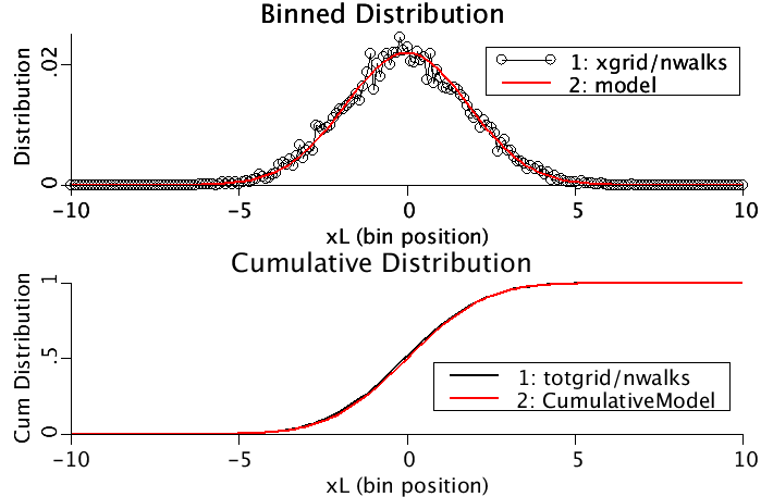
Source: www.physiome.org
The quantum random walk takes this concept and either destroys or improves it, depending on your perspective. We consider that our drunkard is in fact a quantum particle, complete with their own wave function. Instead of a 50\50 ‘coin-flip’ to determine their direction, we instead define an arbitrary ‘coin’ operator that acts on the drunkard’s wave function.
Now, we can define this operator so that it acts the same as the original coin operator, and we define a step operator that shifts the position of the drunkard. After 1 step, our quantum drunkard has a 50% probability of having stepped left or right – but after that, things get a bit hairy. Our quantum drunkard hasn’t actually stepped either left or right, they are in a superposition of states, with half of those states being ones where the drunkard is observed on the left, and half with the drunkard on the right. Because of this, the quantum drunkard’s wavefunction will interfere with itself, combining two overlapping waves into a single big one in some places, and cancelling some out in others.
After a number of steps, the probability distribution looks like this – absolutely not gaussian!
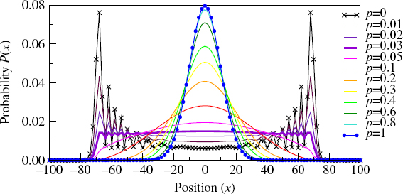
Quantum walks for various values (p) of decoherence. When the decoherence is 1, the walk reduces to a classical random walk. Source: Decoherence versus entaglement in coined quantum walks
I wanted to find a way to visualize what a quantum walk looked like as it was evolving, and how it changed by biasing the coin flip operator. Using Susan Stepney’s very semantic quantum walk code as a base, I wrote a script to generate 3D plots, with the third axis being a parameter of the user’s choice.
First, here is how a our quantum drunkard evolves with time:
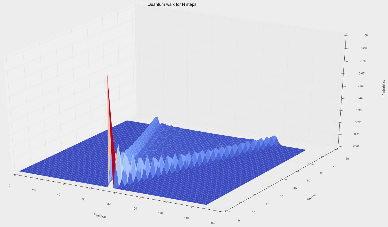
The front of the plot is the first step, and the rear is 80th step. A traditional gaussian would have started as a sharp peak and flattened out over time, but this one splits in two, and spreads out to either side of the distribution like a bow wave
For those who like motion, here is is in motion:
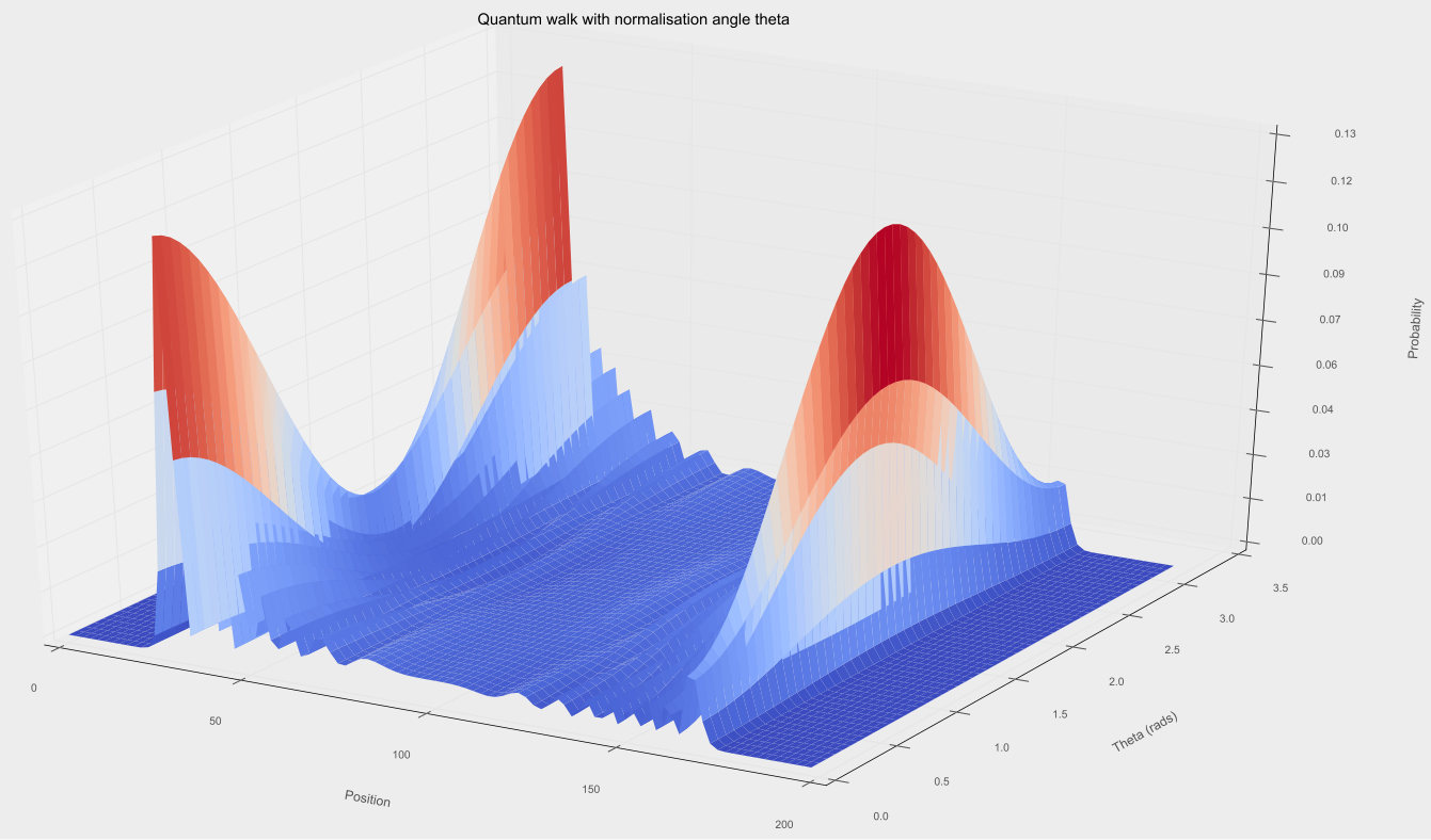
I also tried varying the normalisation constants of the coin operator – biasing the coin to flip one way or the other. This basically meant multiplying the values in the coin operator by trigonometric functions (chosen just because they vary between 0 and 1), which is very evident on the graph:
Quantum random walks might just look like some strange curiosity, but they actually have some interesting uses – mostly in the design of algorithms for quantum computers.
If you’d like to have a play with the quantum random walk code for yourself, you can get it at Susan Stepney’s blog.
Last updated July 19, 2017.